 |
||
|
|
sTCW Differential Expression Guide | |
|
||
- DE per sequence: R scripts for
EdgeR ,DESeq2 .- It is important that you study the documentation for the respective DE method to determine the best approach for your data. You may either use one of the existing scripts, customize an existing script, or create a new one.
- The R-scripts for DE sections explains how
runDE writes the data to R variables, executes the R-script, then reads the results into sTCWdb.
- GO enhancement: R script for
GOseq .- Same comments above. See R-scripts for GO.
Contents:
- Installing R and packages
- Example: demoTra
- DE between conditions
- GO enhancement
- Remove
- R-scripts
- R directory permissions
1. Installing R and packages
Installing R
- See R Project for the latest instructions on installing R.
- See MacOS for installation that worked on MacOS 10.15.
- See R directory permissions for some permission suggestions.
Installing rJava and R packages
- See rJava and R packages.
2. Example: demoTra | Go to top |
From the command line, type:
>runDE tra
Or, if you type
Define a pairwise comparison by selecting "Stem" for
Check the box
Assuming you have installed
Execute The |
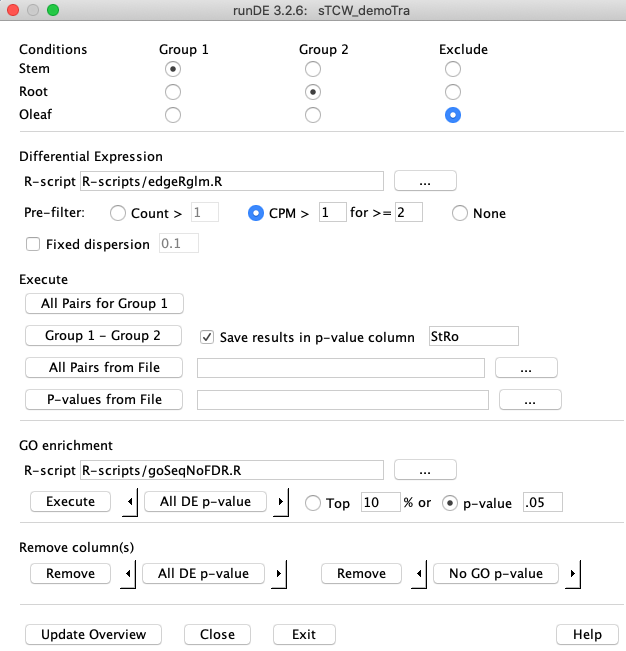
|
Execute DE output
> ****************************************************************
******** Start DE execution for column: StRo *********
****************************************************************
Replicates:
      5 Stem
      5 Root
Collecting count data (may take several minutes)
Using CPM filter > 1 for >= 2
      1 filtered sequences
Assigning R variables
   gc: GC values of sequences
   rowNames: sequences (row) names
   grpNames: group (column) names
   repNames: replicate names
   counts: counts of sequences
   countData <- array(counts,dim=c(210,10))
   rm(counts)
   rownames(countData) <- rowNames
   nGroup1 <- 5
   nGroup2 <- 5

Start R-script
   source('R-scripts/edgeRglm.R')
Loading required package: limma
Using traditional glm (quasi-likelihood F-tests)
   results
   rowNames
R-script done

Number of DE results:
   <1e-5 <1e-4 <0.001 <0.01 <0.05
       6    17    32    65    97

Saving 210 scores for StRo
   Adding column to database...
                            .
Finished DE execution for StRo             0m:0s  (8Mb)
Complete all Group1-Group2 for tra
The console is in R, you may run R commands -- q() or Cntl-C when done, or perform another Execute.
The R console remains open and you can now manually explore the data using R, if desired. However, it easiest to explore it be
selecting "Close" on
	>q()
	Save workspace image? [y/n/c]: y
	R
This saves all variables written by
	> library(edgeR)
	> plotBCV(y)
	> plotMDS(y, labels=grpNames)
Execute GO output
Trace output to stderr and Log file (append): projects/DElogs/tra.log   Size: 11.0kb
****************************************************************
******** 1/1. GO enrichment for column: RoOl *********
****************************************************************
Assigning R variables
  6,651 Numbers GOs
    208 Sequences with GOs from 211 (98.6%)
   seqNames: sequence names
   seqLens:  sequence lengths
   nSeqs <- 211
   seqDEs: DE binary vector (110 p-value < 0.05)
   names(seqDEs) <- seqNames
   seqGOs <- vector("list",nSeqs)
   For all n: seqGOs[[n]] <- c(gonum list)
   names( seqGOs) =  seqNames                       ...

Start R-script
   source('R-scripts/goSeqNoFDR.R')
Using manually entered categories.
Calculating the p-values...
   oResults
   goNums
R-script done

Saving 6,651 values to database
    172 GO p-values < 0.05
Finished GO enrichment for RoOl                                          0m:1s
Summary:
   ColName       #DEseq (%)   DEseq%GO   DEavgLen   DEstdLen     avgPWF     stdPWF     #<0.05
      RoOl      110 (52.9%)      82.3%    1073.89     679.84   0.528607   0.073576        172
Complete GO enrichment for tra
The console is in R, you may run R commands -- q() or Cntl-C when done, or perform another Execute.
The R console remains open and you can now manually explore the data using R, if desired.
However, it easiest to explore it be selecting
	>q()
	Save workspace image? [y/n/c]: y
	R
This saves all variables written by runDE and the script. By restarting R, you can now explore the data for the last enrichment computation, e.g.
	> library(goseq)
	> plotPWF(pwf)
GO output summary
At the end of execution, a summary will be printed to the terminal and log file. For example, if all enrichment p-values are computed for
Summary:
   ColName       #DEseq (%)   DEseq%GO   DEavgLen   DEstdLen     avgPWF     stdPWF     #<0.05
      StRo       97 (46.6%)      80.7%    1075.12     703.22   0.464116   0.000063        311
      StOl      100 (48.1%)      79.5%     991.49     595.44   0.480768   0.065060         48
      RoOl      110 (52.9%)      82.3%    1073.89     679.84   0.528607   0.073576        172
| ColName | The DE column used as input for the GO enrichment. |
| #DEseq (%) | The number of DE sequences for the DE column, where a sequence is DE based on the value
supplied ( |
| DEseq%GO | The percent of unique direct or inherited GOs for the set of DE sequences. Due to inheritance, this tends to be a high percentage. |
| DEavgLen | The average length of the DE sequences. |
| DEstdLen | The standard deviation of the length of the DE sequences. |
| avgPWF | The average of the PWF (probability weighting function). |
| stdPWF | The standard deviation of the PWF. |
| #<0.05 | The number of GOs that have a enrichment p-value <0.05. |
View Results | Go to top |
View DE Results
|
To view the resulting p-values, run ' |
|
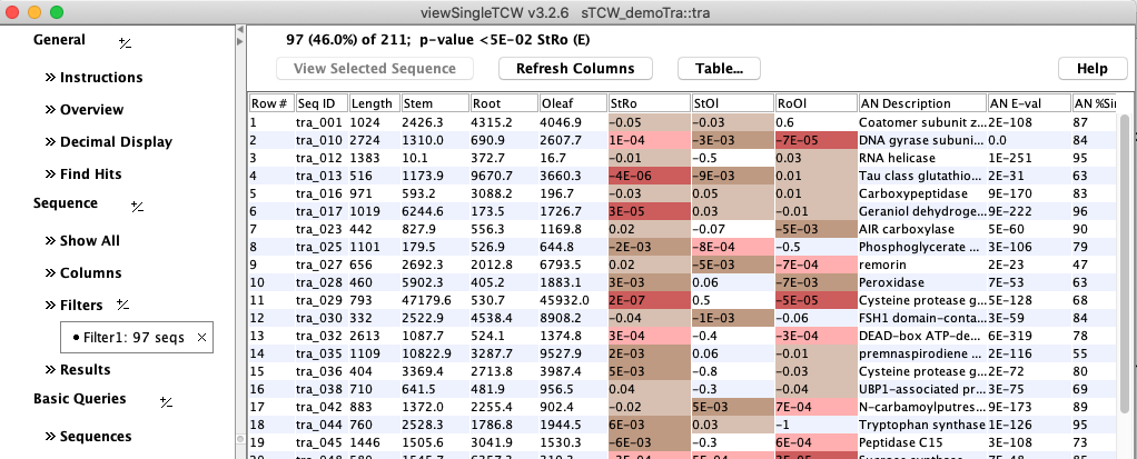
The highlighting and significant digits can be changed in by the Decimal Display panel.
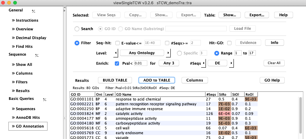
View GO Enhancement Results
3. DE between conditions
Methods & Options | Go to top |
R-script
The default R-script isPre-filter
This example uses a database with 48k sequences and 5 replicates for root and stem. The three filtering options were run with defaults (table on lower left) before input to
2 CPM (Counts per million) = (count/library size)*1M. |
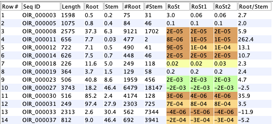
The DE value (RoSt) is set to negative if Root<Stem. The columns prefixed with '#' are the counts, which are used by the filters. The columns with no prefix, Root and Stem, are the TPM values. |
- DE value 3.00: the filtered sequences.
- DE value 2.00: assigned an NA from the DE computation.
To view the first 50 filtered sequences that do not have 'all' zero count values,
execute
e.g.
Using CPM filter > 1 for >= 2, the following shows the first few filtered sequences:
Rep Names       Root1    Root2    Root3    Root4    Root5    Stem1    Stem2    Stem3    Stem4    Stem5
Lib Sizes    25267201 26691329 20806376 24815333 29748103 36131457 25997359 21874134 25691566 31637621
SeqID                                             Counts : CpM
OlR_000003       41   2  16   8   8   7   7   7   4   6  : 1.6 0.1 0.8 0.3 0.3 0.2 0.3 0.3 0.2 0.2
OlR_000016       23   5  37  21  17  26  16  12  13  23  : 0.9 0.2 1.8 0.8 0.6 0.7 0.6 0.5 0.5 0.7
OlR_000053       17  12  10  26  18  30  12  15  25  27  : 0.7 0.4 0.5 1.0 0.6 0.8 0.5 0.7 1.0 0.9
OlR_000063       18   4  21  15  10  24  20  19  24  26  : 0.7 0.1 1.0 0.6 0.3 0.7 0.8 0.9 0.9 0.8
OlR_000066        8   3   1   0   0  20  15  13  34  28  : 0.3 0.1 0.0 0.0 0.0 0.6 0.6 0.6 1.3 0.9
OlR_000083       11  12  13  22  12  11  15   2   3   6  : 0.4 0.4 0.6 0.9 0.4 0.3 0.6 0.1 0.1 0.2
OlR_000100       14   6  21  15  12   7  10   8   2   8  : 0.6 0.2 1.0 0.6 0.4 0.2 0.4 0.4 0.1 0.3
OlR_000162       11  10   7  17   5   8  15   7  18  10  : 0.4 0.4 0.3 0.7 0.2 0.2 0.6 0.3 0.7 0.3
OlR_000181       25   1  24  10   7   6  13   3   4   7  : 1.0 0.0 1.2 0.4 0.2 0.2 0.5 0.1 0.2 0.2
Using Count > 10, the following shows the first few filtered sequences.
SeqID           Root1 Root2 Root3 Root4 Root5 Stem1 Stem2 Stem3 Stem4 Stem5
OlR_000238        4   1   4   1   4   0   0   0   0   0
OlR_000264        8   2   5   2   7   1   0   0   0   1
OlR_000489        0   0   3   0   2   2   1   2   0   1
OlR_000519        0   0   2   0   0   0   0   0   0   0
OlR_000625        5   0   3   2   1   0   1   1   0   1
OlR_000642        7   3   6   4   9   5   4   1   9   8
Fixed dispersion
If there are not biological replicates, then it is necessary to set the dispersion. If it is not set, TCW will use 0.1 by default.
Execute | Go to top |
If multi-condition testing is desired, e.g. to find sequences reduced in condition A compared to
any or all of conditions B,C,D, then the recommended process is to compute the individual
pair DEs A-B, A-C, A-D, and then use filter options in
There are four options to add DE values to the sTCW database, as explained in the following four sections.
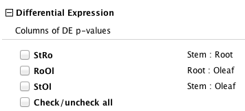
The DE p-value columns will be displayed in
All Pairs for Group 1
- Only check conditions in Group 1.
- Results will be saved in the database with auto-generated column names.
- Execute: Each condition selected in group 1 will be pairwise compared; any selections in Group 2 are ignored.
	Stem  Root   StRo
	Stem  Oleaf  StOl
	Root  Oleaf  RoOl
where the last column is the generated column name.
Group 1 - Group 2
- Select at least one condition from each group.
- If you want to store the results in the database, check
Save results in P-value column . If the groups have been selected, a column name will be auto-generated which you can change. When you change the groups for a subsequent execution, uncheck-then-check the column box to auto-generated a name for the new groups. - Execute: The condition(s) in Group 1 will be compared with the condition(s) in group 2.
All Pairs from File
- Any checked conditions in
Group 1 andGroup 2 are ignored; the conditions to compare are specified in the file. - Results will be saved in the database with the provided column names.
- Execute: All pairs from the file will be compared with the selected method and options.
	Root     Stem  RoSt
	Root     Oleaf RoOl
	Stem     Oleaf StmLea
	Root:Stem Oleaf RoSt_Ol
The last row shows how to select two or more from Group 1; no spaces are allowed between the ":". Group 2 can only have one condition.
Keep the column names short but meaningful. A file similar to the above is in the
P-values from File
The first line defines the two groups and the p-value column name, using the same format as the "Get Pairs from File". All remaining lines have a seqID followed by the p-value. For example,#Example p-value file Root Stem RoSt tra_001 0.14 tra_002 0.14 tra_003 0.65The p-values are read as absolute values since runDE makes values negative if Cond1<Cont2.
4. GO enrichment (over-represented categories) | Go to top |
- R-script: Use the default
goSeqBH.R or supply your own. - P-value columns: If one or more DE p-values have been added to the database, the <---> box will say All p-values; this can be changed to compute GO enrichment for just one p-value column.
- P-value cutoff: A
p-value of 0.05 is the default; this applies to the DE p-value so that all sequences with a p-value<0.05 will be considered DE (which assumes FDR correction was applied). Since the DE p-values still contain considerable uncertainty as absolute measures of probability, there is an option to defined DE in terms of ranking, i.e., top 10% (the ranking is ordered by the p-values).
The result is a p-value column for the GOs, having
the same names as the corresponding sequence DE columns, accessible through the
5. Remove | Go to top |
6. R-scripts | Go to top |
R-scripts for DE
When the Execute is selected, TCW performs the following:- Writes the necessary information to the R environment based on the options selected.
- Runs the R script using the
source command. - Reads the
results variable from the R environment, which should contain the p-values.
	> gc: GC values of sequences
		rowNames: sequences (row) names
		grpNames: group (column) names
		repNames: replicate names
		counts: counts of sequences
		countData <- array(counts,dim=c(210,10))
		rm(counts)
		rownames(countData) <- rowNames
		nGroup1 <- 5
		nGroup2 <- 5
The variables displayed with a ":" after them are assigned with the
The most important variables are
	> head(countData)
			[,1] [,2] [,3] [,4] [,5] [,6] [,7] [,8] [,9] [,10]
	tra_001 1017  594 1222 1209 1315  378 1002 1649  826  1195
	tra_002  272  239  431  400  368  101  206  151  109   185
	tra_003 3830 5185 4847 4857 5451 1859 2506 1334 1541  2307
	tra_004 1707 1088 2429 2210 2334  529  919 1103  810  1427
	tra_005  479  369  439  444  565  114  192  151  232   351
	tra_006 1122  923 1381 1320 1482  632  839  905  670   823
	> grpNames
	 [1] "Stem" "Stem" "Stem" "Stem" "Stem" "Root" "Root" "Root" "Root" "Root"
The R script should put the p-values in the
	> head(results)
	[1] 1.537634e-07 1.695981e-07 2.478791e-07 2.478791e-07 4.026519e-06
	[6] 4.600047e-06
The order should correspond to the input order; if changed, then change the order in
An example script is:
	# edgeR glm method unless no replicates
	library(edgeR)
	y <- DGEList(counts=countData,group=grpNames)
	y <- calcNormFactors(y)
	if (nGroup1==1 && nGroup2==1) {
		writeLines("Using classic with fixed dispersion")
		et <- exactTest(y, dispersion=disp)
		res <- topTags(et, n=nrow(et), adjust.method="BH")
	} else {
		writeLines("Using traditional glm")
		design <- model.matrix(~grpNames)
		y <- estimateDisp(y, design)
		fit <- glmQLFit(y,design)
		qlf <- glmQLFTest(fit,coef=2)
		res <- topTags(qlf, n=nrow(qlf), adjust.method="BH")
	}
	# Columns are:  logFC    logCPM        F       PValue          FDR
	results <- res$table$FDR
	rowNames <- rownames(res)
R-scripts for GO
This works like the R-scripts for DE, with the variables shown below in the GO enrichment example output:
Assigning R variables
  6,651 Numbers GOs
    208 Sequences with GOs from 211 (98.6%)
   seqNames: sequence names
   seqLens:  sequence lengths
   nSeqs <- 211
   seqDEs: DE binary vector (97 p-value < 0.05)
   names(seqDEs) <- seqNames
   seqGOs <- vector("list",nSeqs)
   For all n: seqGOs[[n]] <- c(gonum list)
   names( seqGOs) =  seqNames
The GOs assigned to each sequence are both the direct and indirect.
The p-values to be loaded must be in
The following is the
# goSeq with Benjamini and Hochberg FDR

suppressPackageStartupMessages(library(goseq))
pwf <- nullp(seqDEs,'','',seqLens,FALSE)
GO.wall <- goseq(pwf,'','',seqGOs)
goNums  <- GO.wall$category
oResults <- p.adjust(GO.wall$over_represented_pvalue, method="BH")
FDR
According to the GOseq Manual: "Having performed the GO analysis, you may now wish to interpret the results. If you wish to identify categories significantly enriched/unenriched below some p-value cutoff, it is necessary to first apply some kind of multiple hypothesis testing correction. For example, GO categories over enriched using a .05 FDR cutoff [Benjamini and Hochberg, 1995] are:"> enriched.GO=GO.wall$category[p.adjust(GO.wall$over_represented_pvalue, + method="BH")<.05]Hence, the values loaded into "oResults" for the TCW supplied
oResults <- p.adjust(GO.wall$over_represented_pvalue, method="BH")The p.adjust methods are: c("holm", "hochberg", "hommel", "bonferroni", "BH", "BY", "fdr", "none")
demoTra: The TCW supplied demo result in 0 p-values<0.05.
In order to view some p-values<0.05 results
for the demo, use
Naming R-scripts and Overview | Go to top |
DE (Differential Expression) computation:
      Column       Method               Conditions
      StRo         edgeRglm.R           Stem : Root
      StOl         edgeRglm.R           Stem : Oleaf
      RoOl         edgeRglm.R           Root : Oleaf

   GO enrichment computation:
      Column       Method               Cutoff
      StRo         goSeqNoFDR.R         0.0500
      StOl         goSeqNoFDR.R         0.0500
      RoOl         goSeqNoFDR.R         0.0500
7. R Directory Permissions | Go to top |
Unless you plan to run as root (not recommended),
or will be the only one running
When you install an R package, it can go either to a shared location or to a user-specific location.
Installing to the shared location is better, as others can then use the package, however in the default
installation of R the shared directories are owned by the root user and their permissions must be
changed to allow ordinary users to install shared packages. This is done as follows (unless you have
- Run R (by typing "R")
- In R, use
Sys.getenv("R_HOME") to find the R installation directory (usually /usr/lib64/R) - Exit from R with command "q()"
-
ls /usr/lib64/R (or wherever the R_HOME was) - The directory listing should have a
library subdirectory; if not, R is not installed right - Change permissions on the
library directory (and everything under it) such that ordinary users can write to it. Ideally there is an appropriate user group and you can usechgrp -R <group> library andchmod -R g+w library to give this group write permissions. Otherwise,chmod -R 777 library will be necessary.
| Email Comments To: tcw@agcol.arizona.edu |