FPC V8: A tutorial
F. Engler and C. Soderlund
Arizona Genomics Computational Laboratory
BIO5 Institute, University of Arizona, Tucson AZ 85721
Corresponding author: cari@agcol.arizona.edu
April 2006
This manuscript is modified from “FPC: A software package for physical maps”, In Ian Dunham (ed) Genomic Mapping and Sequencing, Horizon Press, Genome Technology series. The introduction has been removed, and the manuscript has been edited by William Nelson in order to update it to FPC V8.0. This work was funded by USDA/IFAFS grant #11180
We have written this tutorial to cover the salient features of FPC. It is augmented by FPC help, which can be accessed by most of the FPC windows. It can also be accessed as an HTML file from http://www.agcol.arizona.edu/software/fpc/FPChelpdoc.htm. This tutorial covers the features we used to build the maize physical map -- that is, incrementally assembling the map, ordering contigs based on framework markers, adding markers and remarks, and searching. Other than merging and adding remarks, we will not cover any editing functions as these are nearly obsolete. If needed, they are covered in the User’s Manual.[1] We briefly describe comparing multiple gel images using the Gel Image window. This feature is used in selecting a MTP, which is covered by Humphrey and Mungall (2002). (Note that FPC version 7 and later contains an automated MTP selection function).
Table of Contents
Analysis.............................................................................................................................. 3
Tolerance and cutoff......................................................................................................... 3
CB maps and CB units................................................................................................. 3
Q clones........................................................................................................................... 5
Getting started................................................................................................................... 6
Some Unix basics............................................................................................................ 6
Installing FPC.................................................................................................................. 6
Downloading the demo files............................................................................................ 6
Building a physical map with FPC.................................................................................. 6
Creating a new project................................................................................................ 6
The DQer....................................................................................................................... 10
Incremental Builds......................................................................................................... 11
Adding remarks and markers........................................................................................ 12
Manually adding remarks............................................................................................... 12
Adding remarks and markers from a file........................................................................ 13
Searching.......................................................................................................................... 15
Finishing a project........................................................................................................... 18
Merging Contigs............................................................................................................ 18
Adding singletons.......................................................................................................... 20
Verify overlap................................................................................................................ 21
BIBLIOGRAPHY........................................................................................................... 25
Analysis
We
will start out describing the major aspects of analysis. You may want to skip
this and come back to the various sections when they are referenced during the
tutorial. We assume that the reader is familiar with the fingerprinting
technique by restriction digest (Marra et al. 1997).
Tolerance and cutoff
The
bands of two clones are compared to determine the probability that the two
clones overlap by chance. The FPC assembly algorithm uses two user-defined
variables for measuring clone overlap: tolerance and cutoff. The tolerance determines how closely
two bands must match to consider them the same band. If you are using migration rates, a fixed tolerance is used;
that is, the same tolerance is used regardless of the value. If you are using
sizes, a variable tolerance is generally used; see Soderlund et al. (1997a).
The probability that the matching bands are just a coincidence is computed, and
the cutoff value is a threshold on the probability score. If the result of the
equation is below the
cutoff, the two clones are said to overlap, i.e. the matching bands are less
likely to be a coincidence. The cutoff is expressed in scientific notation: a
1e-03 is the same as 0.001 and 1e-05 is 0.00001. A higher exponent is a lower
score; a lower score is a higher stringency. We will usually refer to a high or
low stringency when discussing the cutoff value. The equation that is used for
comparing two clones is stated as follows:
![]()
where p = (1 – b)nH, b = 2t/gellen, t is the tolerance, gellen is the number of possible values for bands, nL and nH are the minimum and maximum number of bands for the two clones (nL<nH), and M is the number of shared bands. Since the tolerance is used in the equation, it is desirable to set it at the beginning of your analysis and never change it; a change requires reassembly of the entire database. Since the number of bands is also used in the equation, two clone pairs with the same number of matching bands may have two very different probabilities of coincidence (see Table I).
|
Number of Bands |
|
|
|
|
Clone 1 |
Clone 2 |
Matching Bands |
Prob. of Coin. |
|
52 |
38 |
12 |
3e-02 |
|
52 |
16 |
12 |
3e-06 |
Table I. Number of Matching Bands Versus the
Probability of Coincidence. Even
though the two clone pairs have the same number of matching bands, they have
different probabilities of coincidence.
CB maps and CB units.
FPC
orders overlapping clones and puts them into contigs based on the probability
of coincidence scores. As it
orders the clones, it tries to order the bands to provide a more precise
definition of the endpoints of clones.
As shown in Soderlund et al. (2000), better data yields more precise
endpoints. Even with the high quality data being produced today, much ambiguity
remains: (1) two bands may have the same length, but be different, (2) two
bands may have values where the difference is outside the tolerance, but be the
same, (3) bands may be missing, and (4) there may be extra bands, for example,
many digests result in end bands. Therefore, slippage occurs in the endpoints;
but unless the data is of especially low quality or contains Q clones (as
described in the next section), clones that are supposed to overlap based on
the cutoff do overlap. Also, the algorithm is greedy -- that is, to save time,
it does not try all possible combinations, and therefore cannot guarantee the
best solution. It tries a number of different solutions, each time starting
with a different clone, and takes the best one (the number to try is adjustable
by the user but defaults to 10).
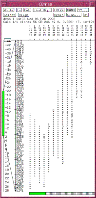
|
Figure 1. A CB map displayed in FPC. The consensus bands are shown along the left. The tick marks represent partially
ordered groups. The {+,x,o} character columns represent the clones. A ‘+’ indicates a match with the
band to the left within the tolerance, a ‘x’ indicates a match within twice
the tolerance, and a ‘o’ indicates no match. The number of extra bands for
each clone is listed under the clone name. |
The ordering of clones and their
fragments is called a Consensus Bands (CB) map, an example of which is shown in
Figure 1. The coordinate system
used in the contig display is in CB units: each distinct band is one unit of measurement. The length
of each clone is equal to the number of bands in the clone. Endpoint
coordinates are assigned as follows: N is equal to the number of bands in the clone divided by 2, M is the midpoint of the location of the
clone in the CB map, M-N
is the left coordinate of the clone and M+N is the right coordinate of the
clone. The left endpoint of the
contig is set to zero, but can go negative. Note that the coordinates do not
have any meaning relative to the chromosome until they are mapped by a
framework marker.
Q clones
A
large number of Q clones generally result from one or more false positive
overlaps. Say clone x
from contig A falsely
overlaps with a clone y
from contig B. As clones are being added to the CB map
from contig A, when
clone x is added, it
brings in clone y,
which in turn brings in all of contig B. Since there is no way to provide a linear order for two
contigs in the same space, the clones in the second contig end up in a stack
(see Figure 2). The CB map software recognizes that it cannot order the bands
for these clones, and consequently marks them as Q clones. In assembly, a low stringency cutoff
results in contigs with many Q clones (i.e. many false positives); a high
stringency cutoff results in too many contigs (i.e. many false negatives). Empirical evidence shows that for BAC
clones with an average of 28-35 bands, a 1e-12 cutoff works well to minimize
the number of contigs and contigs with many Q clones. Note: It is not unusual
to have a few Q clones in a contig due to poor fingerprints or as a result of
the greedy nature of the assembly algorithm
|
Figure
2: Contig with Q clones: the stack of clones in the center indicates an F+ overlap. |
Getting started
Some Unix basics
FPC
runs under Unix and Linux. An
extensive knowledge of Unix is not necessary to use FPC effectively. Users must know how to logon to a
Unix terminal, and perhaps have a basic knowledge of the directory
structure. In this tutorial, any
necessary commands are given as they are used. Two basic commands to know are cd,
which changes a directory, and ls, which lists all files in the current
directory.
Installing FPC
If
FPC is not installed on your system, ask your system administrator to download
an FPC executable from http://www.agcol.arizona.edu/software/fpc and place it
in a shared area for all users to access.
Currently, executables for Solaris, Linux, and Mac are provided. If none of these match your machine
type, you will need to have your system administrator download the source code
and compile an executable in order to run FPC.
Downloading the demo files
Download demo.tar from
http://www.agcol.arizona.edu/software/fpc. When this file has finished downloading, type tar xvf demo.tar on the command line and press return. This action creates a directory called demo
in your current directory. Type cd demo to
move into that directory. Then
type ls. The following
files should be listed:
copyNew.pl /files /Image /Sizes
cleanup.pl /Gel Newbands
Image, Sizes, and Gel are
directories, and the files in them are generated from the Image program (see
www.sanger.ac.uk/Software/Image). NOTE: if at any time during the tutorial you
wish to bring the demo back to its initial condition, type cleanup.pl
on the command line while in the demo directory. This will restore all files and directories back to their
original condition so you can restart the demo from the beginning.
Building a physical map with FPC
Creating a new project
The commands
covered in this section:
- Create new project (File...)
- Update .cor
- Build Contigs (from
Main Analysis window)
- Buried clones and contig navigation
- Clean up
From
the demo directory, start FPC by typing fpc
on the command line. The Main Menu
window appears (see Figure 3).
Right-click on the button labeled File… and a menu appears.
Select Create new project from the menu and a window appears as is
shown in Figure 4. Choose a name
for your project and type it in the File: text entry. For this demo, type the name “demo”. Click OK; a demo.fpc
file is created, and the following is written to the terminal window:
Serial implementation
Adding Bands Directory
Configuration file demo.fpp not found. Therefore will use
defaults.
New project is initalized.
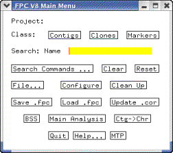
|
Figure 3: The Main
Window. This is the first window you will see when you start FPC. |
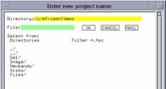
|
Figure 4: From the File… menu, choose Create
new project, and this window appears. Enter a name. |
Now
click on the Update .cor button on the Main Menu window. This function moves all migration rate
files from the Image directory to a newly created Bands
directory.[2] It also creates the file demo.cor,
which is the file FPC uses to read the migration rates of clones. When this function has completed, the
last few lines written on your terminal window will be (with your path name
substituted for /u/efriedr):
Read 311
files. Add 345 gel entries and 9456 bands.
Cor file
has 9456 bands.
Saving
File /u/efriedr/demo/demo.fpc ......Done
Click
on the Main Analysis button on the Main Menu window and the
Main Analysis window opens (see Figure 5).
Figure 5: Main Analysis
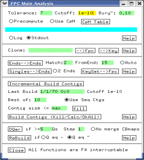
Change
the cutoff to 1e-12 in the Cutoff text box. Leave all other values
unchanged. Next, click on the Build Contigs (Kill/Calc/OkAll) button. This starts the map-building process. This process may take several hours for
large clone libraries, but for the demo, it should only take a few
seconds. When this process
completes, the last few lines on your terminal window will be:
Complete Build: Tol 7 Cut 1e-12 Bury~ 0.10 Best 10
Singles 5 AvgOverlap 3.8 AvgScore 0.871 Qs 30(1) (<=5Qs 0 >5Qs 1)
Create 4 contigs (1:4): Max 121, 3 (>50), 1 (50:26), 0
(25:4), 0 (3:2)
NxN Pairs: Real time 0.140s User time 0.150s Sys time 0.000s
Layout:
Real time 0.540s User
time 0.510s Sys time 0.000s
Note,
the number of Qs may be 30 or 31, and the times will vary. The Project window
pops up, as shown in Figure 6a.
The assembly resulted in four contigs. Double-click on the row of contig 2 and it is displayed, as
shown in figure 7.
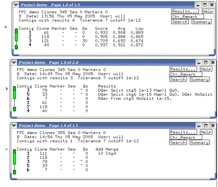
Figure 6. The Project window.
(a) Shows the window after an initial build, (b) after the DQer was run,
and (c) after new clones were incorporated and the IBC was run. Note the change in Q clones from (a) to
(b), and the merging of contigs from (b) to (c).
Not
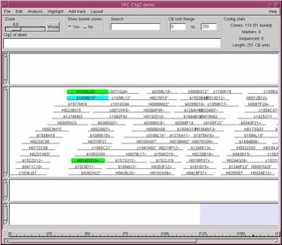
all the clones are shown as redundant clones are buried. Click the button called Yes underneath
the Show buried clones label and all the clones are shown (see
Figure 7). If a clone has a set of bands similar to another, it can be buried
in the second clone. Click on a clone that has an "*" at the end of the clone
name; the "*" implies that it has buried clones and the buried clones are
highlighted. A clone ending with a "=" has all the same bands as the parent
clone. A clone ending with a "~" has approximately the same set of bands as the
parent clone. Click on the No button again to switch back to the
buried state. You can zoom by
holding the mouse down on the slider within the ruler under the Zoom
label, and moving one way or another; alternatively, you can click in the grey
area of the ruler. To scroll around the contig display, move the mouse pointer
towards the right of the map and click on the middle mouse button (feature not
available on two-button mouse).
The map scrolls to the left.
To move back, position the pointer towards the left of the map and
click. You can alternatively use
the ruler at the bottom of the display.
|
Figure 6. The Contig display.
The Yes was selected under Show buried clones, so all clones are
shown. Selecting a clone shows the buried clones highlighted green |
To close all windows at once except the
Main Menu window, select Clean Up on the Main Menu.
The DQer
Commands covered
in this section:
- The DQer (from
Main Analysis)
- Save .fpc
Open
the Project window by double-clicking on the bold-faced project name (demo) at the top of the main menu. Look at
the column with the heading ‘Qs’ on the Project window. Notice that three contigs have a 0 in
this column, while contig 3 has a 30. (Contig 0 contains all clones that could
not be placed in the map; hence, Q clones do not apply.) After an initial build with a moderate
cutoff, we need to take the contigs with many Q’s and re-run them at a lower
cutoff. The DQer performs this
function automatically. Click the Main
Analysis button from the
Main Menu. Towards the bottom you
will see a button labeled DQer with two text entries to the right of it. The first text box (if >= 5 Qs)
determines how many Q’s a contig must have in order to be re-evaluated. Empirical evidence has shown that a
value around 5 yields good results. The second text box (Step 1) is relevant
for HICF (see the HICF tutorial www.agcol.arizona.edu), and will be ignored for
this demo. Click on the DQer button and the reanalyzation starts. The contigs with Q’s above the cutoff
are reassembled up to three times, with cutoffs of 1e-13, 1e-14, 1e-15. The
software tries to merge the CB maps by comparing the end clones at a lower
stringency. If the CB maps cannot be merged, one or more new contigs are
created. When the DQer is done, the
Project window pops to the front, as shown in Figure 6b. A contig with many Qs
may not change if lowering the cutoff 3-fold does not make a difference; that
is, when all clones remain in the same contig and the number of Qs remains
high. This indicates contamination or a very repetitive fingerprint.
Save
the current contigs by clicking on the Save
.fpc button on the Main Menu
window. The ONLY time the FPC
project is automatically saved is after an Update .cor. Therefore, whenever you have made some
changes that you want saved, do so immediately. You can save any number of
times during an FPC session. The benefit of saving often is that if you make a
mistake (e.g. merge two contigs) and then decide you did not really want to do
that, you can quit and restart FPC from your last save. Select the Quit
button on the Main Menu to exit FPC.
Type ls on the command
line to see the new files created by FPC.
The following should now be listed:
Bands/ demo.cor.backup files/ Sizes/
cleanup.pl demo.fpc Gel/
copyNew.pl demo.fpc.backup Image/
demo.cor demo.fpp Newbands/
Incremental Builds
Commands covered
in this section:
- Adding additional clones to an
existing FPC project.
- Incremental Build Contigs (IBC, on Main
Analysis window)
We
will now add some additional clones to our FPC project. Generally, as new gels
are band-called, Image places the files in the Image, Sizes,
and Gel directories. For this demo, a new set of files was
temporarily put into the Newbands directory, and the files can be moved to
the correct locations using the copyNew.pl perl script. From the demo directory,
type ./copyNew.pl on the command line to copy the files
from the Newbands directory into their respective Image,
Gel, and Sizes directories. Thereafter, launch FPC with the previously created project
(we called it “demo”) by typing fpc
demo on the command
line. When the Main Menu window
appears, click on the Update .cor button. This will copy the files from the Image
directory to the Bands directory, and it updates the demo.cor
file with the new migration rates.
We are now ready to add the new clones to our map. Open the Main Analysis window. The
cutoff should still be set at 1e-12. Click on the Incremental Build Contigs button. This adds the new clones to our map and merges contigs if
the new information allows us to do so.
When the build is done, the Project window will pop to the front (see Figure
6c). Contigs 1 and 4 have been
merged indicating that one or more of the new clones hits both. Save the new map by clicking on the Save .fpc
button on the Main Menu.
Adding
remarks and markers
Manually adding remarks
Commands covered
in this section:
- Finding a clone in a contig
- Editing the clone
Open
the Contig display for contig 2 (via the Project window). At the top, in the text entry labeled Search,
type b0297K22 and hit
Return. The clone is found in the
contig, so it will be highlighted as shown in Figure 8a. Click on the
highlighted clone and the Clone window opens (see Figure 8b). Click on the Edit
button in the top left corner and the Edit Clone window opens (see Figure 8c). Here we can change the attributes of
the clone, including attaching remarks.
In the text entry titled Remarks, type test_remark to add that remark to the clone. Click on Accept Edit. The Clone Edit window closes, and our
newly added remark in the Clone text box. It is also shown in the Contig
display; clicking on the clone highlights the remark and vice versa. Select Clean up
on the Main Menu before going on to the next section.
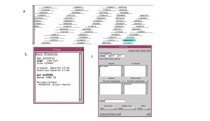
Figure 8. (a) Click the highlighted clone to bring up the Clone text window. (b) The Clone text window. (c) The Edit Clone window.
Adding remarks and markers from a file
Commands covered
in this section:
- Merge remarks (from Main Menu/File menu)
- Replace markers (fw & seq) (from Main Menu/File menu)
- Framework (from Project
window)
- By framework order (from Project window/Menu window)
Often remarks can be generated from an external file, in which case it is faster to automatically add them all at once. Hence, FPC provides features for adding a list of remarks from an external file. The text file is a list with entries such as the following:
BAC : "b1046D08"
Remark
"new_add"
Look
at remarks.ace in the files directory for
an example. In addition to clone
remarks, remarks may be added to markers and to contigs, using very similar
file formats and commands. Examples of marker remark and contig remark files
are also located in the files directory.
To
add the clone remarks, on the Main Menu right-click on the File… button
and select Merge clone remarks from the drop down menu. This opens the File Chooser
window. Double-click on files/
in the left-hand column. Then
double-click on the remarks.ace file that appears in the right-hand column. This action adds all remarks in the remarks.ace
file to our project. These
particular remarks note which clones were added after the initial build by
adding the remark new_add
to those clones. Open the contig
display for contig 1 to see where the remarks were placed.
A
typical scenario for markers is that the clone/marker results are entered into
a simple marker database or spreadsheet. A perl script is written to convert
the format to the FPC marker file format. As markers are incrementally added to
the spreadsheet, all markers are periodically dumped and input into FPC using
the Replace markers function. The advantage of replacement
is that any deleted markers or markers removed from clones from the external
marker database, are also deleted in FPC. Each time the marker file is read, if
a framework file exists, it is also read. This is a file of ordered markers,
generally from a genetic or radiation hybrid map, which orders the contigs. As
new markers are added, this file is re-read to see if any new frameworks can be
added; a framework marker can go into FPC only if it is attached to a clone.
The markers file is structured like the remarks file; see markers.ace
file for an example. Each framework file uses the same name as the marker file,
with the .ace suffix replaced with .fw.
Each entry contains four items[3]:
1) marker name, 2) chromosome or linkage group, (3) marker position, and 4) F
or P for framework (well ordered) or placement (not well ordered). To read in the markers and framework
file, right-click on File… on the Main Menu and select Replace markers (fw & seq).
From the File Chooser window, double click markers.ace. The markers and framework (called markers.fw)
are read into our project. When this completes, open the Project window and
right-click on the button in the top right corner titled "By
ctg...". Select Framework
from the menu. The framework
markers are shown in order, and the contigs containing these markers are shown
in the rightmost column, as shown in Figure 9a.
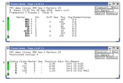
Figure 9. (a) Lists the frameworks (alias
anchors). The F indicates a framework, while no F indicates a placement. (b)
The contigs after they have been assigned a chromosome and reorderd.
Select the J130 marker from the framework project window
and select ctg5 from
the Marker text window (see Figure 10a). The framework markers are shown along
the bottom of the contig display, while all framework and non-framework markers
are displayed along the top (see Figure 10b). Even when only a small region of
the contig is displayed, all framework markers are always shown along the
bottom. You can center on the region of a framework by clicking on it in the
bottom part of the display.
To re-order the contigs so that they are
ordered according to the framework markers, select Ctg->Chr
on the Main window[4];
a window appears, select Assign
Ctg->Chr followed by Order Ctgs based on Chr assignment.
The results are shown in Figure 9b.
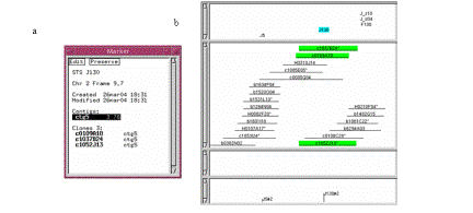
Figure
10. (a) Marker window. (b) The markers are displayed towards the top
of the window, while the framework is displayed along the bottom.
Searching
Commands covered
in this section:
- Select keyset type: Contigs,
Clones, or Markers
- Search by substring of name
- Search by remark
- Search by date
- Add remark to all clones in the
keyset
- Keyset
(from Edit Contig window) – show clones from keyset in contig.
- Configure Display (from Contig display) – turn on Fp_remarks.
Using
aceDB terminology, there are three classes of data in FPC: contigs, clones, and markers. A subset of a
class can be shown as a keyset
of items. The three buttons on the Main Menu, labeled Contigs,
Clones, and Markers, determine which class is searched. A class is selected for searching by
clicking on the corresponding button, which highlights it in blue. Once a
keyset is displayed, the next search of that class is performed on the existing
keyset. Consequently, you can search for multiple conditions; e.g. first search
for all clones added after a given date, and then search that keyset for all
clones in a given contig.
Select the Contigs class. On the Main Menu is the label Search:, next
to this is the search type, by default
Name, and next to this is a
text box. Type a 1 in the text
entry and press return (or click on the Contig button). Contig 1 is shown.
Select Clear and the text in the Search text box will
disappear. Double click the Contigs
class; all the contigs will be shown in the keyset. All remaining contig
searches are from the Project window from the button titled "Search".
Select the Markers class and
type A07 in the text
box. The marker window for that
marker pops up. Double click on
the bold-faced contig number (ctg1)
to see where the marker is positioned.
Next, select Clear and then type A* in the Search text entry. This brings up the Keyset window
containing a list of all markers starting with the letter A. Double-clicking on any marker name will
bring up the Marker window for that marker.
Select the Clones class and
search for clone c1086K04,
which will open the Clone window.
Once again, double-click on the contig number to see the position of the
clone in the contig. Next, select Clear
then type b*. This brings up a keyset containing all
clones starting with b. To see
the distribution of b clones among all contigs, open the Project window,
right-click on the upper right button (labeled By ctg...), select By keyset. This gives us the number of b clones
in each contig sorted in descending order. Now, suppose that we want to see all clones in contig 1 that
start with b. Open contig 1 from
the Project window. Click on the Highlight button at the upper left corner, and
from the menu choose Select Keyset. All b clones are selected, i.e. shown
in blue. Figure 11 shows us the relation between the Keyset, Project, and
Contig windows.
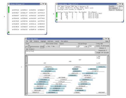
Figure 11. Viewing keysets in the Contig display. (a) The keyset shown is a subset of all
the clones. (b) The Project window displays the number of clones from the
keyset that are in each contig.
Double-clicking on the row for contig 1 brings up the Contig
display. (c) From the Select Contig
window (from Edit button), click on Keyset to select all clones from the keyset
that are in contig 1. (d) All
clones from the keyset in contig 1 are selected (blue).
Our next search involves searching for
clones containing the new_add
remark that we attached to all clones added after the initial build. First, reset the keyset to all clones
in the project by selecting Reset from the Main Menu. Right-click on the Search Commands… button and select Remark from the menu. In the text entry, type new_add.
The Keyset window gives us all ten clones containing that remark. Looking at the keyset values in the
Project window shows us that all of our new clones were added to contig 2. Open that contig display and from the Edit
button, select Select Clones, then select Keyset. All
new clones will be selected in the contig display.
Our final search involves searching for
clones by date and time. We will
find all clones that were added after the initial build by searching for all
clones that were created after a specified time. Since the creation time of the added clones is very close to
the creation time of the initial clones (unless you added the initial clones
one day, and the additional clones on a subsequent day), we need to include the
time when specifying the date.
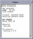
Reset the clone keyset to show all clones. Double click the first
one. It does not have the remark new_add; note the creation date and time of this
clone. On the Main Menu, select After Create Date from the Search
Commands… menu. In the Search text entry, type in the
date and time such that the time is at least one minute AFTER the creation time
of the clone. Type the date and
time in the format dd/mm/yy hh:mm.
(Note: this is the European date format - the day comes first.) Press return. For example, in Figure 12, the created day and time is
18feb02 19:50 so we would enter the time as 18/2/02 19:51. The Keyset
window opens listing all clones created after this date and time. Select a
clone and make sure it has the new_add remark. Now, suppose that we want to add a remark to the
two clones in this set that start with an H. Without closing the Keyset window, select Name
from Search Commands on the Main Menu. In the Search text entry, type H*.
Now, only those clones from the former set that started with an H are
shown in the keyset. Right-click
anywhere in the white space on the Keyset window, and select Add Remark
from the pull-down menu. The Add remark
window pops up. Type in any remark
up to ten characters long and click on Add
Fp_remark. Next, double-click on one of the clones
in the keyset, and then double-click on the bold contig number in the Clone
window to open the Contig display. Fp_remarks are typically less important, so
are generally made invisible by editing the remark track (see contig display
demo).
Figure 12. Clone Text Box Shows a Remark and a
Fp_remark. The display of these in
the contig display window can be turned on or off by right-clicking in white space
within the contig and selecting Edit Track Properties. See the Contig
Display tutorial, available at
www.agcol.arizona.edu/software/fpc,
for more information.
With the left button, select Search Commands.
The Clone Commands window containing various types of searches is shown. Many
of these are intuitive. The ones we use most are Multiple Fingerprints,
which show all the clones that have multiple gels (none in this set). The Selected
option makes a keyset of all the selected clones in the current contig, where a
clone can be selected by clicking on its name with the right button and then
clicking Selected. The selected set can be cleared by
clicking Clear All on the contig window.
Finishing
a project
Merging
Contigs
Commands covered
in this section:
- Ends-Ends (Main
Analysis window)
- CpM table (Cutoff plus
Markers for scoring overlap, Main Analysis window)
- Merge (Contig
display)
After
the majority of the data is entered into FPC, it is advantageous to find
contigs that can be merged. An
easy way of finding candidates for merging is to lower the stringency and only
compare clones close to the ends of contigs. Lower the stringency by setting the cutoff to a 1e-10. We
will use the CpM table to help us identify contigs to merge. When this table is used, clones that
share one or more markers can have a less stringent cutoff and still be
considered overlapping. On the
Main Analysis window, turn on the CpM table by clicking on the radio button
labeled Use CpM.
On the terminal window, you will see:
Cutoff 1e-10 CpM (1 1e-9)(2 1e-08)(3 1e-07)
This
information is also shown on the CpM window, which you can view by clicking CpM Table.
Note: We generally turn the CpM table on from the beginning of the project. As
new clones and markers are added to FPC, the IBC (Incremental Build Contigs)
takes into consideration new markers and reanalyzes those clones with new
markers for joins.
On the Main analysis window, change the
number beside Match to 1.[5]
Click on the Ends-Ends
button. When this finishes, the
Project window pops up showing us suggesting that contigs 1 and 3 can be
merged, as well as 3 and 5. The “RR-1
ctg3” in the comment for contig 1 means that
one clone from the right end of contig 3 overlaps with one clone from the right
end of contig 1. Open the Contig
display for contig 1 and click on the Merge Contigs option
of the Edit button at the top. The Merge contig window opens (Figure
13a). If the merge remark was LR
or LL, the first contig would need to be flipped, in which case, you would
select the first Flip button and it would immediately be flipped. Since the
merge remark has an R for the second letter, we need to flip Ctg3. Enter a ‘3’ next to Ctg, select Flip
and click on Start merge.
Contig 3 is appended to contig 1 as is shown in Figure 13c. Notice the
clones from contig 3 are in a lighter font indicating that they are not
permanently part of contig 1. Select marker F100 and you will see that it is in
a clone in contig 1 and a clone in contig 3. Also, a window appears (see Figure
13b) allowing us to move the two contigs closer together or farther apart. Click on the arrows to move the
contigs. A value of –20 gives
a reasonable merge. This can be
checked by either of the methods described in the Verify overlap section. When you are done, click on Accept merge. The two contigs permanently become
one.
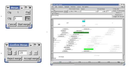
Figure 13. (a) Choose which contig to merge. (b) Move the merged contig. (c) The merged contig is in a lighter font.
We
have just merged contig 1 onto the right end of contig 3, but recall that Ends-Ends also reported a possible merge of
contig 5 to the same end of contig 3. Usually it does not make sense to merge
two contigs to the same end of third contig, so further study would be needed
in this case to determine which, if any, of the merges to perform. This could
involve building the CB maps for the merged contigs (see FPC notes from the FPC
web site), checking the banding pattern explicitly (see below), or using
additional information such as markers or synteny with a reference species.
Note that no CB map has been computed for
the merged contigs. The contigs were simply joined at their ends, using the
merge distance specified in the "Confirm Merge" dialog. Because the
CB was not recomputed, the number of Q clones is not known accurately, and the
best FPC can do is to add the Q clones from the two contigs prior to the merge.
In this case the result is 0, and it is listed as "~ 0" on the
Project page (see By_ctg), where the "~" indicates that the value has
not been accurately computed. The reason the CB map is not automatically
recomputed is that manual merges generally are found at less-stringent cutoffs,
and assembling even a good contig at a less-stringent cutoff can result in
errors, since clones may have false-positive overlaps with other clones in the
same contig. CB maps for all "~" contigs may be recomputed using the
"ReBuild" button on the Main Analysis page,
and for a specific contig the CB map may be computed by using the "Compute CB Maps..." option from the Analysis menu on the
contig display page.
Now re-run Assign Ctg-Chr as any addition or removal of clones
from the contig causes the assignment to be invalid. Note that we merged two
contigs that had frameworks from different chromosomes, hence, it can no longer
be assigned to a chromosome.
Adding
singletons
Commands covered
in this section:
- FPC-Ctgs (from
Main Analysis window)
- Show additions (from Contig Analysis window)
There
are times when we want to add clones to our map, but we do not want to merge
any contigs. For example, after all data is added and manual merges have been
completed, we do not want merges to occur automatically anymore; therefore, we
cannot run the IBC. Another time this is used is towards the end of a project
when singletons are
added at a lower stringency and should not be used for merges (a singleton is a
clone that has not been placed in a contig). Hence, FPC provides the capability
to add singletons to contigs if there exists an overlap with one or more clones
in a contig, without doing any merges. The clone is positioned where the best
overlap occurs. Users should be
warned not to use this function inappropriately; a low stringency cutoff value
can add many clones to the map, but they could be positioned incorrectly as
there is no global analysis taking place. From the Main window, select Clones
to make it the current keyset. Select Search
Commands using the left
mouse so that the Search Command window will appear. Select Singletons.
The word 'Singletons' should appear on the Main Window. On the Main Analysis
window, set the cutoff to 1e-10, turn on the Auto radio button,
and click on the KeySet->Fpc button. All singletons that overlap clones already in a contig at
this lower stringency are automatically added to the contig. When the function completes, the
Project window pops up, showing us in which contigs our singletons found
overlapping clones. The number in
the Results column gives us the number of clones
that overlap our singletons at the lower stringency. Open the Contig display for contig 1. Click on the Highlight
button at the top of the window and choose the Show Additions
option. All newly added clones are
highlighted in dark blue, so clones H0278N12 and H0125D1, along with several others, should be highlighted in dark
blue[6].
The added clones may be buried, in which case toggle the buried state to see
them.
Bring up the Project window and select By Ctg from
the pull-down menu in the top right corner. Note that the number of Qs for contig 1 and contig 2 are set
to ‘~ 0'; this is again because the number of Q clones is not accurately known
since the CB maps have not been recomputed with the added clones. These contigs
can be reanalyzed as described above, but this is not usually necessary unless
there is reason to believe some of the singletons were incorrectly placed.
Also, the Chromosome assignments have been cleared; once again, run Assign Ctg->Chr.
Verify
overlap
Commands covered
in this section:
- Clone 1-Ctg CpM
(from Contig Analysis, compare clone 1 against contig)
- From Clone text window, bring up Gel
Image window
- Gel Image window,
add and move clones
- Clone 1-Clone 2
(from Contig Analysis, compare two clones)
When
clones are added at a lower stringency and are not positioned with the
automatic analysis, there is greater risk of a false positive or poorly
positioned clone. Therefore, it is worth verifying the addition by looking at
the raw fingerprints. It takes a while to become an expert at looking at gel
images, but we will take you through one to get you started. First, we will
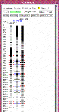
compare the fingerprint of clone H0278N12 with its immediate neighbors. Locate the clone in the
Contig 1 display and click on it to select it. Then open the Evaluate window
from the Analysis menu. Clicking
on the Clone 1 button in this window copies the
selected clone name to the first text entry. Next, click on the →Ctg CpM button. The overlapping clones are highlighted
in purple and the following text is displayed on your terminal window:
>> --> Ctg1 H0278N12 28b 32 60 (Tol 7 Cutoff 1e-10 CpM NoBuried)
c1021A24 ( 27, 64) 38b 20
3e-11
b1537B07 ( 31, 65) 35b 19
9e-11 canon
Right-click
on clone H0278N12 and
select Gel image from the pull-down menu. The Gel image
window shown in Figure 15 appears. The tick marks on both sides of an image is
the ‘called bands’ for the clone.
The numbers along the left side are the scale for migration rates. We need to determine if this banding
pattern is similar to that of its neighbors. Bring up the images of the clone’s immediate neighbors (b1537B07 and c1021A24) by turning on the Add
button in the Gel Image window by clicking on it, and then clicking on the
neighbor clones in the contig display.
The images for the clicked clones will appear in the Gel Image window. Turn off Add by clicking on
the button again. Now, we will
position the clones in the Gel Image window such that our selected clone is
flanked by its two neighbors. Turn
on Move and arrange the gels by dragging and dropping the images
such that clone H0278N12
is in the middle. Then turn off Move. Next, click on the name of our newly
added clone in the Gel Image window. All bands that have matches with the neighbors are colored in
blue, while bands that are not matched remain black. On the neighbors, any bands that match are shown in
red. You can also zoom in and out
as desired by clicking on the corresponding buttons at the top of the Gel Image
window. Zoom out a couple of times
to view a similar image as is shown in Figure 15. The GreyRamp tool adjusts the
contrast of the gels. If the
banding pattern seems plausible, we can keep this clone. The method of analyzing the
fingerprints is discussed in greater detail by Humphrey and Mungall (2002).
Figure 15: Gel Image
window
Quit out of the Gel Image window. On your
terminal window are the results of the previous clone comparison. Put the
cursor beside the text c1021A24, hold down the left button, and drag the
cursor over the name. Put the cursor in the yellow box beside Clone 2
on the Contig Analysis window and click the middle button and the text will be
dropped into the yellow box. Using this technique, text can be dragged and
dropped into any text box in FPC. Select →Clone 1. Select the Size
radio button to turn it on. On your terminal window, the last few lines will
say:
Olap 28
Match 11 1e-03 (Nsizes 28 38)
Total
size overlap 50239 Shared markers
0
Olap
28 means that the two clones
overlap by 28 CB units. Note that it says they have an overlap of 1e-03, but
previously it said these two clones match based on a cutoff of 1e-10. The
following is happening: FPC notes that there is a Size
directory, so it reads the size value for these clones and compares them with a
variable 0.007 tolerance. It also determines the physical overlap based on the
variable tolerance, which is approximately 50239 bases. Furthermore, it gives
the total sizes for each clone at the beginning of this printout (i.e. 126163
and 168382). Click on the Size radio button to turn it off. Hit
→Clone 1
again. Now the output is:
Olap 28 Match 20 3e-11 (Nbands 28 38)
Total band overlap 20893 Shared markers 0
Now
the output is using bands. The fixed tolerance 7 on bands finds more shared
ones than a variable tolerance 0.007 on sizes. The Size option is there so that
you can see the sizes and is not practical for matching unless the variable
tolerance value has been optimized.
Summary
From the Project window, you can view the
results in different ways. We have already looked at the Framework window. To
see the length of the contigs in CB units, go to the Project window, pull down
on the upper right button, and select By
Length. Pressing the Summary
button shows you the average number of bands per clone and other statistics
(see Figure 16).
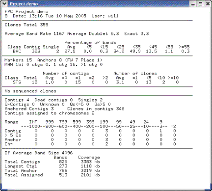
Figure
16: From the Project window,
select Summary.
Additional
FPC Menus
We
have only touched on a few of the many functions available through the Edit and
Analysis menus of the contig display window. These functions allow detailed
editing and analysis of contigs, and they are all documented through the Help
buttons on the respective windows. It is well worth experimenting with the
functions in these menus and reading their help pages.
A
number of other useful functions are found on the Search and
Cleanup menus. The Search menu is reached directly by clicking Search on
the project page, and the Cleanup menu is a button at the bottom of the Search page.
These functions are not fully documented but many are self-evident.
BSS
and FSD
BSS (BLAST Some Sequence) is a function built in to FPC which makes it easy to locate sequences on the FPC map, if the clones on the map already have some associated sequence, e.g. BAC end sequences (BES). BSS takes any other sequences (e.g. marker or draft genomic sequences) and blasts them against the clone-associated sequences. BSS consolidates the BLAST output into an interactive report and can then add the results to FPC as markers or remarks. This has been extremely valuable in mapping genetic markers and draft sequence to the rice FPC map, which helps anchor contigs, closes gaps, and select a minimal tiling path. See the BSS tutorial from the FPC web site.
We have also developed the tools FSD (FPC Simulated Digest) and FSD2 to perform simulated agarose fingerprinting on a sequenced clone; the resulting in silico fingerprint can be automatically assembled into FPC. This can help to close gaps and anchor contigs, and having the sequenced clones located on the FPC map also provides more targets for BSS searches, as described above. FSD thus has a synergistic relation with the BSS: as more sequence is added, more electronic markers can be mapped.
Parallel FPC
Many FPC operations are computationally intensive, and therefore have been parallelized in order to allow maximum speed on today's increasingly-common multiprocessor machines. To run fpc version 8.0 using N processors, launch it as follows:
fpc -p N myfile.fpc
FPC
will then use all N processors for CPU-intensive tasks such as building contigs
or CB maps.
Building HICF maps
HICF (High Information Content Fingerprinting) is becoming increasingly prevalent, and requires certain adjustments to FPC. These are covered in detail in the HICF tutorial available on our site.
Other documentation
Besides
the documentation provided through the Help
buttons on FPC itself, there
are several other useful tutorials and references available on our web site, http://www.agcol.arizona.edu/software/fpc.
These include tutorials on the contig display, on BSS, and on using FPC to
build HICF (High Information Content Fingerprint) maps. Please feel free also
to send us email with any questions.
BIBLIOGRAPHY
Altschul,
S.F., Madden, T.L., Schaffer, A.A., Zhang, J., Zhang, Z., Miller, W., and
Lipman, D.J. 1997. Gapped BLAST and PSI-BLAST: a new generation of protein
database search programs. Nucleic
Acids Research. 25: 3389-3402.
Chen,
M., Presting, G., Barbazuk, W., Goicoechea, J., Blackmon, B., Fang, G., Kim,
H., Frisch, D., Yu, Y., Higingbottom, S., Phimphilai, J., Phimphilai, D.,
Thurmond, S., Gaudette, B., Li, P., Liu, J., Hatfield, J., Sun, S., Farrar, K.,
Henderson, C., Barnett, L., Costa, R., Williams, B., Walser, S., Atkins, M.,
Hall, C., Bancroft, I., Salse, J., Regad, F., Mohapatra, T., Singh, N., Tyagi,
A., Soderlund, C., Dean, R., and Wing, R. 2002. An integrated physical and
genetic map of the rice genome. Plant Cell.
Coe,
E., Cone, K., McMullen, M., Chen, S., Davis, G., Gardiner, J., Liscum, E.,
Polacco, M., Paterson, A., Sanchez-Villeda, H., Soderlund, C., Wing, R. 2002.
Access to the maize genome: an integrated physical and genetic map. Plant
Physiology. 128: 9-12.
Ding,
Y., Johnson, M., Colayco, R., Chen, Y., Melnyk, J., Schmitt, H., and Shizuya,
H. 1999. Contig assembly of bacterial artificial chromosome clones through
multiplexed fluorescent-labeled fingerprinting. Genomics. 56: 237-246.
Durbin,
R., and Thierry-Mieg, J. 1994. The AceDB Genome Database. (ed. Suhai, S.),
Computational Methods in Genome Research. Plenum Press, New York, pp.
7821-7825.
Engler,
F., J. Hatfield, W. Nelson, and C. Soderlund (2003). Locating sequence on FPC
maps and selecting a minimal tiling path. Genome Research 13:2152:2163. PDF
Supplemental
Engler,
F. and C. Soderlund (2002). FPC: A software package for physical maps. In Ian
Dunham (ed) Genomic Mapping and Sequencing, Horizon Press, Genome Technology
series. Norfolk, UK, pp. 201-236.
Hoskins,
R., Nelson, C., Berman, B., Laverty, T., George, R., Ciesiolka, L., Naeemuddin,
M., Arenson, A., Durbin, J., David, R., Tabor, P., Bailey, M., DeShazo, D.,
Catanese, J., Mammoser, A., Osoegawa, K., de Jong, P., Celniker, S., Gibbs, R.,
Rubin, G., and Scherer, S. 2000. A BAC-based physical map of the major
autosomes of Drosophila melanogaster. Science. 287: 2271-2274.
Marra,
M., Kucaba, T., Dietrich, N., Green, E., Brownstein, B., Wilson, R., McDonald,
K., Hillier, L., McPherson, J., and Waterston, R. 1997. High throughput
fingerprint analysis of large-insert clones. Genome Research. 7: 1072-1084.
Marra,
M., Kucaba, T., Sakhon, M., Hillier, L., Martienssen, R., Chinwalla, A.,
Crockett, J., Fedele, J., Grover, H., Gund, C., McCombie, W., McDonald, K.,
McPherson, J., Mudd, N., Parnell, L., Schein, J., Seim, R., Shelby, P.,
Waterston, R., and Wilson, R. 1999.
A map for sequence analysis of the Arabidopsis thaliana genome. Nature
Genetics. 22: 265-275.
Mungall,
A. and S. Humphrey (2002). Assembling physical maps and sequence clone
selection. In Ian Dunham (ed) Genomic Mapping and Sequencing, Horizon Press,
Genome Technology series. Norfolk, UK, pp. 167-200.
Nelson,
W. and C. Soderlund. Software for restriction fragment physical maps. In K.
Meksem, G. Kahl (ed) The Handbook of Plant Genome Mapping: Genetic and Physical
Mapping, Wiley-VCH, p. 284.
Nelson,
W.M., A.K. Bharti, E. Butler, F. Wei, G. Fuks, H. Kim, R.A. Wing, J. Messing,
and C. Soderlund. 2005. Whole-genome validation of high-information-content
fingerprinting. Plant Physiol
139: 27-38.
Pampanwar,
V., F. Engler, J. Hatfield, S. Blundy, G. Gupta, and C. Soderlund. 2005. FPC
Web tools for rice, maize, and distribution. Plant Physiol 138: 116-126.
Soderlund,
C., Longden, I., and Mott, R. 1997a.
FPC: a system for building contigs from restriction fingerprinted
clones. CABIOS 13: 523-535.
Soderlund,
C., Gregory, S., and Dunhum, I. 1997b. Sequence ready clones. (ed. M. Bishop)
Guide to Human Genome Computing. Academic Press. pp. 151-177.
Soderlund,
C. 1999. FPC V4.0: User's Manual. Technical Report SC-01 -99. The Sanger
Centre, Hinxton Hall, Cambridge UK.
Soderlund,
C., Humphrey, S., Dunham, A., and French, L. 2000. Contigs built with
fingerprints, markers and FPC V4.7. Genome Research. 10: 1772-1787.
Soderlund,
C., Engler, F., Hatfield, J., Blundy, S., Chen, M., Yu, Y., and Wing, R. 2002.
Mapping sequence to Rice FPC. In
C. Wu, P. Wang, and J. Wang (ed). Computational Biology and Genome Informatics.
Selected papers from CBGI 2001. World Scientific Publishing.
Sulston,
J., Mallet, F., Staden, R., Durbin, R., Horsnell, T., and Coulson, A. 1988.
Software for genome mapping by fingerprinting techniques. CABIOS. 4: 125-132.
The
International Human Genome Mapping Consortium. 2001. A physical map of the
human genome. Nature. 409: 934-941.